DESCRIPTION

The elementary comparison test ( ECT) is a thorough technique for the detailed testing of the functionality. The necessary test basis is pseudo-code or a comparable specification in which the decision points and functional paths are worked out in detail and structurally.

The ECT aims at thorough coverage of the decision points and not at the combining of functional paths. The basic technique used here is Decision points: modified condition/decision coverage.

• Decision points: multiple condition coverage. With this, the possibilities within the decision points (specifically selected, if necessary) can be tested in more depth.
• Boundary value analysis. With this, the possibilities within the decision points (specifically selected, if necessary) can be tested in more depth.
• Pairwise testing. With this, the testing of possible combinations of functional paths is added.

It is a preferred technique for testing functions deemed very important and/or complex calculations.

POINTS OF FOCUS IN THE STEPS

In this section, the elementary comparison test is explained step by step. In this, the generic steps (see Test Design Techniques) are taken as a starting point. An example is also set out, showing at every step how this technique works.

Example 1 - In this example, we take a function (task) in which the data referring to the car owner are entered in a screen and subsequently, upon request, a calculation is made of the premium that the car owner should pay for his vehicle insurance. Depending on a number of variables, the level of the premium is established. The pseudo-code below gives a detailed functional description of this:

IF Age < 18 years OR driving licence suspended THEN Error message
ELSE IF Age < 25 years AND years holding driving licence < 3 THEN Premium := 1,500
ELSE Premium := 800
ENDIF
IF Car age < 2 OR (car age ≥ 5 AND damage in last 3 years ≥ 2,500) OR age ≥ 70 THEN Increase premium by 500
ENDIF
ENDIF

It is set out per step below how the elementary comparison test is applied to this function:

1 - Identifying test situations

The test basis consists of pseudo-code or a comparable formal function description which can be copied directly in this step. If not, an extra activity should be carried out in order to convert the existing specifications into pseudo-code.

The decision points in the pseudo-code are provided with unique identification. It is usual to use the codes D1, D2, etc. for this (or D01, D02, etc. if there are many decision points).

Example 2 - There are three decision points, which are shown structurally below:

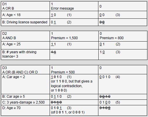
NB! In D3, the combination “A = true and B = true” gives a logical contradiction and therefore may not occur in the test situations: Car age should be simultaneously lower than 2 and higher than, or equal to, 5. This contradiction would otherwise show up when the test cases are made physical.

Detailed working out of the derived test situations:


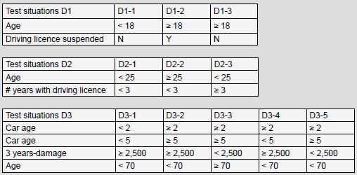
NB! The parameter “Age” occurs in the decision points D1, D2 and D3. This leads to the following mutually exclusive test situations: D2-1 with D3-3; D2-3 with D3-3.

Graphic demonstration of test situations

For some testers, the creation of logical test cases is made easier with the aid of a graphic demonstration of the test situations – a Graph.

With this, each decision point and end point is represented by a circle and each test situation by a line that goes from one circle to another. A logical test case runs through the graph from beginning to end, linking a chain of test situations. The graph also supplies insight into the minimum number of test cases necessary to cover all the test situations. This is determined by the maximum number of parallel lines in the graph.

Example 4 - The test situations are reproduced in figure 1:


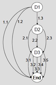
Figure 1: Graph with test situations for ECT

2 - Creating logical test cases

A test case runs through the functionality from start to end and will come across one or more decision points on its path. With each decision point, the test case will test one of the defined test situations.

The logical test cases are combined with the aid of a matrix. The rows contain the test situations and the columns contain the logical test cases. With each test case, it is indicated by one or more crosses which test situations should be tested by this test case. This matrix simultaneously serves as a check on the complete coverage of test situations.

In order to take account of the nesting of decision points, the columns “Value” and “Next” have been added. These indicate for each test situation what the outcome of the decision is (directly obtainable from the tables in step 2) and to which subsequent decision point (or end process) this leads. This helps to prevent the tester from placing a cross at a test situation where the test case does not go.

Example 5 - Table 1 describes test cases TC1 to TC7 included, which give the required coverage:

Table 1: Logical test cases for ECT.

Mutually exclusive test situations

Each test situation sets particular requirements on one or more parameters. If a parameter occurs in several decision points, it is possible that a test situation in one decision point sets requirements on that parameter that conflict with the requirements of a test situation in another decision point. For example, test situation D2.1 requires “Age < 25” and test situation D3.3 requires “Age ≥ 70”. These test situations are mutually exclusive.

A logical test case may not contain “mutually exclusive test situations”, for that makes the test case inconsistent and therefore unexecutable. Such a test case will be discovered automatically, as soon as the test case has to be made physical (see next step). The problem can then be simply resolved, by replacing one of the “mutually exclusive test situations” with a non-conflicting test situation. In this connection, it can be advantageous to first translate each logical test case into a physical test case in order to discover possible mutually exclusive test situations, before starting on the following logical test case.

• Inventory which parameters occur in several decision points, and (per parameter) which decision points they are
• Sum up the combinations of mutually exclusive test situations.

• Each column describes a physical test case.
• The first row indicates per test case which test situations should be covered.
• Thereafter, there is a row for each parameter of which the test case consists.
• Finally, one or more rows are added with which the predicted result is described in concrete terms.

Example 6 - In table 2 the physical test cases are shown, including the predicted results:

Table 2: Physical test cases for ECT.

4 - Establishing the starting point

No remarks.

Example 7 - The premium sums should be entered in the database. The details of the car owner are entered online and the premium is then calculated immediately.